From leg-joint to tyssue, a refactoring story - Ep. 1

Intro

So I’m giving a talk at EuroScipy at the end of the summer (hooray!). It is based on the code I developed to model fold formation in the drosophila leg imaginal disk, which was published earlier this year. A lot as moved since I submitted the abstract. So here are some thoughts on what happened, and what motivated the switch to a new, more generic library.

Here is the submitted abstract (I’m all about code re-use)

Biological tissues, and more particularly epithelia are very particular kinds of material. Not only do they behave like solids and liquids at the same time (think shaving foam), they are also governed by the behavior of their constituent individual cells. Biological processes (a bunch of incredibly complex chemical reactions) and physics are intertwined so that complex forms emerge from initially smooth tissues.

Along advanced imaging techniques and genetic manipulation of model organism, biophysical modeling is key in understanding these shape changes, or morphogenesis. We studied the role of programmed cell death, or apoptosis in the formation of a fold in the fruit fly pupae (an intermediate stage between larva and adult). In a recently published article we demonstrated that apoptotic cells had an active role in shaping this fold (which will later become a joint in the adult fly’s leg). Cells die on a ring around the socket shaped tissue (one cell thick, and about 200 µm in diameter), they contract and pull on their neighbors, initiating changes in the tissue properties.

In this presentation, I will describe how we use python to develop a numerical model of this epithelium. The leg-joint module is based on Tiago Peixoto’s graph-tool library, and uses SciPy optimization routines to perform the gradient descent at the core of the dynamical simulation. The following topics will be discussed:

• Visualization: plain matplotlib vs vispy vs Blender.

• Performance: can we go from 24 hrs per simulation to less than 1? The pure python vectorization and BoostPython/CGAL routes.

• Future plans: towards a biological tissue physics engine.

The code is showcased in a series of Jupyter Notebooks that can be browsed here.

The three points above deserve some developments, so I’ll do 3 posts, not in the original order, though.

1. Performance - this post
2. Future plans - not so future anymore - next post
3. Visualization (where I’m least advanced) - the third one

The pitfalls of research driven developments

The leg_joint code was developed while our understanding of the biology was progressing at a fast pace, as Magali’s team accessed new genetic tools and gradually improved the fluorescence microscopy images of the drosophila’s leg disk. That left little room for API design, or optimization. I went for results straight ahead, tried to document and test, though not enough, but my time was well spent in maths (that bloody gradient), biology and getting correct figures.

For the published version, getting a simulation of the full fold formation process takes about 24 hours on a single core, which is not sustainable …

Optimization

So I started refactoring once the paper was published. The performance bottleneck was quite obvious: the gradient descent code was called locally (only on a group of cells) a lot of times to mimic a global epithelium relaxation, and this code contained explicit loops over each cell of the global patch to update geometry and gradients at each optimization step. This is bad, but was easy to write. It also made whole tissue optimization depressingly slow. As a good SciPythonista (if that’s a thing), I started looking at vectorization strategies.

I started using graph-tool for its efficient management of dynamic graphs and graph drawing capacities. In this library, values attached to vertices and edges can be accessed as Numpy arrays through the get_array attribute of the PropetyMap class. But as the documentation warns:

The returned array does not own the data, which belongs to the property map. Therefore, if the graph changes, the array may become invalid and any operation on it will fail with a ValueError exception. Do not store the array if the graph is to be modified; store a copy instead.

Furthermore, you can only set the ‘true’ values of the property map for the all array at once. Said otherwise, you can’t use fancy indexing to set values of a given variable (e.g. the x coordinate) of a subset of the graph’s vertices directly, you have to modify a copy of the array and feed it back to the PropertyMap.

You can access a subset of the graph through filtering, i.e. defining a binary mask over the network. But filtering is not the same as indexing, for example you can do this with indexing:

import numpy as np
a = np.arange(4) + 2
b = a[0, 1, 3, 3, 3]
print(b)
>>> [2, 3, 5, 5, 5]

But you can’t tell a mask to repeat a value, and that was exactly what I needed to compute my epithelium geometrical properties. With PropertyMaps, you can get values from fancy indexing, but setting them back is more complicated, due to the rather convoluted way graph-tool mirrors the underlying C++ data and the property map .a attribute, that returns a numpy array. Of course graph-tool was not meant for that kind of computation, it’s focus is on graphs’ topology, not geometry or calculus.

The cell’s area is a good example for the type of computation I was trying to run. It is computed as the sums of the cell’s sub-faces areas, which are themselves half the norm of cross product of two sub-face vectors:

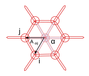
The area of the sub-face is \(A_{\alpha ij} = || r_{\alpha i} \times r_{\alpha j} || / 2\).

Cross product works just fine with numpy 2D arrays, but to compute it, I need to repeat each vector twice for each adjacent face, sum over the cells, and put this back in the property map holding the cell area, for future use. Hence my indexing issue with graph-tool property maps. This motivated the passage to pandas DataFrames to do the geometrical computing. Fancy indexing is what pandas is made for, isn’t it?

Here is an outline of the strategy I used to gather the data from the graph’s property maps and turn them into DataFrames:

1. First find all the triangular faces in the graph, using graph-tool’s subgraph_isomorphism, and get the indices of the 3 vertices (two junctions and a cell).

2. Use this as a MultiIndex to instanciate a DataFrame holding a copy of the relevant data.

3. Do the maths.

4. Feed back the data to the graphs’ property maps.

Thanks to graph-tool, the first point is easy to achieve, and quite fast (like some seconds for a full 2000 cells simulation):

def get_faces(graph, as_array=True):
    '''
    Retrieves all the triangular subgraphs of the form
       1 -- > 2
        ^   ^
         \ /
          0
    In our context, vertex 0 always corresponds to a cell
    and vertices 1 and 2 to junction vertices

    Parameters
    ----------
    graph : a :class:`GraphTool` graph instance
    as_array: bool, optional, default `True`
      if `True`, the output of `subraph_isomorphism` is converted
      to a (N, 3) ndarray.

    Returns
    -------
    triangles:  list of gt.PropertyMaps or (N, 3) ndarray
      each line corresponds to a triplet (cell, jv0, jv1)
      where cell, jv0 and jv1 are indices of the input graph.
    '''
    tri_graph = gt.Graph()
    ## the vertices
    verts = tri_graph.add_vertex(3)
    ## edges
    tri_graph.add_edge_list([(0, 1), (0, 2), (1, 2)])
    _triangles = gt.subgraph_isomorphism(tri_graph, graph)
    if not as_array:
        return tri_graph, _triangles
    triangles = np.array([tri.a for tri in _triangles], dtype=np.int)
    return triangles

This works thanks to the definition of the graph edges, with edges from cell center to junction vertices always oriented outwards, such that the triangular pattern uniquely defines the set of faces.

The triangles array then served as a MultiIndex for a pandas DataFrame called faces. Each of the vertex index was repeated as many times as necessary, and it was then easy to pick the correct data to compute the desired crossproduct, and do sums for each cells (something like faces['sub_areas'].sum(level='cell')).

According to git log, it took me about three weeks to vectorize completely the geometry and gradient computation, but the effort was worth it, with a time gain about two orders of magnitudes (unfortunately, I didn’t document properly the successive gains in computing time), close to the 24 to 1 hours goal I bragged about in the abstract, at least on a relatively simple test case. At that point, “all” that was left was the fourth point of the list above.

Refactoring

But then… I spent the next two months (!) trying to integrate back my new faces DataFrame within the general framework. The main hurdle comes when the graph topology changes, which creates indexes mis-alignments and synchronization nightmares. Maybe it’s my fault for not doing this at the proper level, or not specifying things more clearly; alternatively, graph-tool is not that adapted to 3D geometry computations and it’s time for some new API design.

So at the beginning of May, I decided to reboot the project, and started working on tyssue. As this post is already too long, I’ll discuss this on the next one.